Generating halo and galaxy populations with DiffmahPop and DiffstarPop

This notebook gives a basic illustrations of how to use DiffmahPop and DiffstarPop withing the diffsky pipeline to generate a catalog of simulated mass accretion histories and star formation histories.

%matplotlib inline

Matplotlib is building the font cache; this may take a moment.

import numpy as np
from matplotlib import pyplot as plt
import matplotlib.gridspec as gridspec
from matplotlib.patches import Patch
from matplotlib.lines import Line2D
from scipy.optimize import curve_fit
mred = u"#d62728"
morange = u"#ff7f0e"
mgreen = u"#2ca02c"
mblue = u"#1f77b4"
mpurple = u"#9467bd"

colors = [mpurple,mblue,mgreen,morange, mred]

import subprocess


def try_enable_latex():
    """Try enabling LaTeX text rendering in matplotlib,
    fallback if not available."""
    try:
        # Quick check: can we run latex?
        subprocess.check_call(
            ["latex", "--version"],
            stdout=subprocess.DEVNULL,
            stderr=subprocess.DEVNULL,
        )
        plt.rc("text", usetex=True)
        plt.rc("font", family="serif", size=22)
        plt.rc('figure', figsize=(6,4))
        print("LaTeX rendering enabled.")
    except (subprocess.CalledProcessError, FileNotFoundError):
        # LaTeX not installed or failed
        plt.rc("text", usetex=False)
        plt.rc("font", family="serif", size=22)
        plt.rc('figure', figsize=(6,4))
        print("LaTeX not available, falling back to default mathtext.")

try_enable_latex()

LaTeX rendering enabled.

from jax import jit as jjit
from jax import numpy as jnp
from jax import random as jran
from jax import value_and_grad

# Some constants
from dsps.constants import T_TABLE_MIN
from diffstar.defaults import LGT0 as DEFAULT_LGT0
TODAY = 10**DEFAULT_LGT0

Generate a simulated halo catalog with diffmahpop

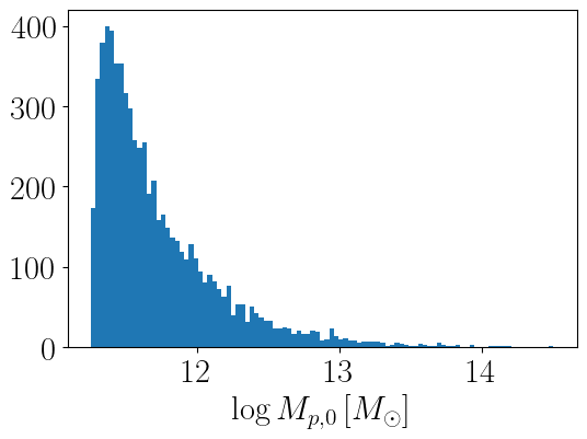
Here we generate a simulated Monte Carlo realization of a subhalo catalog at a single redshift using the diffmahpop wrapper in the diffsky pipeline.

The DiffmahPop model is a generator of mass accretion histories for a population of haloes, using the diffmah model.

Please note that the diffmahpop wrapper within the diffsky repo is likely to change in the future, since it is in a development stage.

from diffsky.mass_functions.mc_diffmah_tpeak import mc_subhalos

ran_key = jran.PRNGKey(0)

# Generate a random subhalo catalog
subcat_key, ran_key = jran.split(ran_key, 2)
lgmp_min = 11.25
z_obs = 0.01
Lbox = 75.0
volume_com = Lbox**3
subcat = mc_subhalos(subcat_key, z_obs, lgmp_min=lgmp_min, volume_com=volume_com)

plt.hist(subcat.logmp0, np.linspace(lgmp_min, 14.5, 100))
plt.xlabel(r"$\log M_{p,0}\,  [M_{\odot}]$")
plt.show()

Load DiffstarPop parameters fitted to different simulations

DiffstarPop has a set of default parameters, but it also has a set of parameters that best-fit three different types of simulations:

• The hydrodynamical simulation IllustrisTNG.

• The semi-analyitical model (SAM) Galaticus.

• The empirical model UniverseMachine.

These can be accessed through the diffstar.diffstarpop.kernels.params module.

They can be used to place informed priors from galaxy formation models into the SFHs of galaxies.

from diffstar.diffstarpop import DEFAULT_DIFFSTARPOP_PARAMS
from diffstar.diffstarpop import SIMULATION_FIT_PARAMS
print(SIMULATION_FIT_PARAMS.keys())

# These are fit for in-situ only SFHs.
DIFFSTARPOP_UM = SIMULATION_FIT_PARAMS["smdpl_dr1_nomerging"]
DIFFSTARPOP_TNG = SIMULATION_FIT_PARAMS["tng"]
DIFFSTARPOP_GALCUS = SIMULATION_FIT_PARAMS["galacticus_in_situ"]

# These are fit for in-plus-ex-situ SFHs.
DIFFSTARPOP_UM_plus_exsitu = SIMULATION_FIT_PARAMS["smdpl_dr1"]
DIFFSTARPOP_GALCUS_plus_exsitu = SIMULATION_FIT_PARAMS["galacticus_in_plus_ex_situ"]

odict_keys(['smdpl_dr1_nomerging', 'smdpl_dr1', 'tng', 'galacticus_in_situ', 'galacticus_in_plus_ex_situ'])

Calculate the SFHs using the UniverseMachine params

Here we calculate the MAH from the halo parameters that we previously generated.

We generate star formation histories for each halo. A galaxy in a given halo can be in the main sequence or quenched, with a certain probability given by the quenching fraction. We generate both, along with the frac_q that each halo might be quenched. We also generate a monte-carlo realization for the halo catalog, assigning whereas each halo is hosting a main sequence or quenched galaxy, via mc_is_q.

from diffmah.diffmah_kernels import mah_halopop
from diffstar.diffstarpop import mc_diffstar_sfh_galpop
from diffstar.defaults import FB as DEFAULT_FB


# Create a table of times where to calculate the MAH and SFH
ntimes = 50
tarr = np.linspace(T_TABLE_MIN, TODAY, ntimes)

# Calculate the mass accreation history of every halo
dmhdt_fit, log_mah_fit = mah_halopop(subcat.mah_params, tarr, DEFAULT_LGT0)

# Manually set the infall data of each halo to no infall,
# since this part of the Diffstarpop model has not been calibrated

n_halos = subcat.logmhost_ult_inf.shape[0]

lgmu_infall = -1.0 * np.ones(n_halos)
logmhost_infall = 13.0 * np.ones(n_halos)
gyr_since_infall = -99.0 * np.ones(n_halos)

# compute SFHs for the default galaxy population
args = (
    DIFFSTARPOP_UM,
    subcat.mah_params,
    subcat.logmp0,
    subcat.upids,
    lgmu_infall,
    logmhost_infall,
    gyr_since_infall,
    ran_key,
    tarr,
)

(
    diffstar_params_ms,
    diffstar_params_q,
    default_sfh_ms,
    default_sfh_q,
    frac_q,
    mc_is_q,
) = mc_diffstar_sfh_galpop(*args, lgt0=DEFAULT_LGT0, fb=DEFAULT_FB)

# select at random if a galaxy is MS or Q based on frac_q.
default_sfh = np.zeros_like(default_sfh_ms)
default_sfh[mc_is_q] = default_sfh_q[mc_is_q]
default_sfh[~mc_is_q] = default_sfh_ms[~mc_is_q]

Make some plots

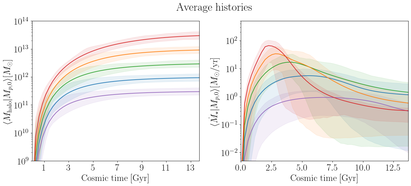
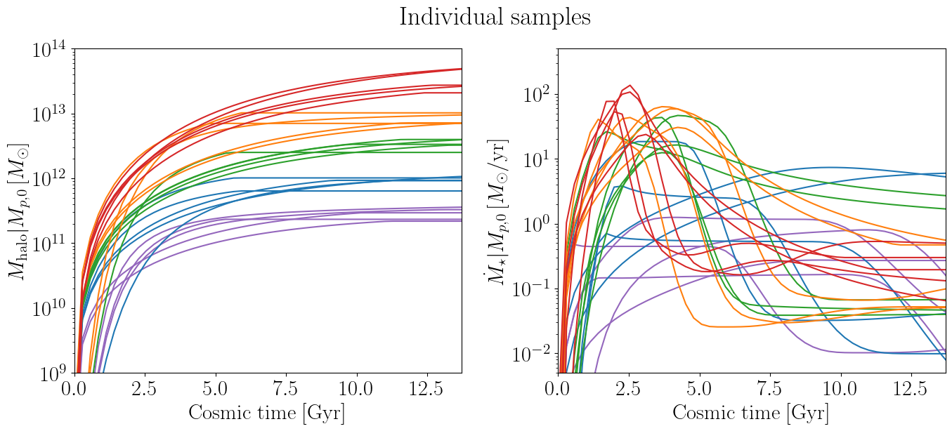
Here we plot the average MAH and SFH histories we have generated, for halos of different present-day halo mass.

We also plot a few individual MAH and SFH histories.

fig, ax = plt.subplots(1,2, figsize=(16,6))
mpeak_vals = np.arange(11.5, 14, 0.5)
for i, mpeak in enumerate(mpeak_vals):
    sel = (subcat.logmp0 > mpeak - 0.2) & (subcat.logmp0 < mpeak + 0.2)
    mean_log_mah_fit = np.mean(log_mah_fit[sel], axis=0)
    mean_default_sfh = np.mean(default_sfh[sel], axis=0)
    range_log_mah_fit = np.percentile(log_mah_fit[sel], [15.865, 84.135], axis=0)
    range_mean_default_sfh = np.percentile(default_sfh[sel], [15.865, 84.135], axis=0)

    ax[0].plot(tarr, 10**mean_log_mah_fit, color=colors[i])
    ax[0].fill_between(tarr, 10**range_log_mah_fit[0], 10**range_log_mah_fit[1], color=colors[i], alpha=0.1)
    ax[1].plot(tarr, mean_default_sfh, color=colors[i])
    ax[1].fill_between(tarr, range_mean_default_sfh[0], range_mean_default_sfh[1], color=colors[i], alpha=0.1)


ax[0].set_ylim(1e9, 1e14)
ax[0].set_xticks(np.arange(1.0, 14.0, 2.0))
ax[0].set_xlabel("Cosmic time [Gyr]")
ax[1].set_xlabel("Cosmic time [Gyr]")
ax[0].set_yscale('log')

ax[0].set_xlim(0.0, 13.7)
ax[1].set_xlim(0.0, 13.7)
ax[1].set_yscale('log')
ax[1].set_ylim(5e-3, 5e2)
ax[1].set_ylabel(r"$\langle \dot{M}_\star | M_{p,0} \rangle [M_{\odot}/{\rm yr}]$")
ax[0].set_ylabel(r"$\langle M_{\rm halo} | M_{p,0} \rangle [M_{\odot}]$")

fig.subplots_adjust(wspace=0.25)
fig.suptitle("Average histories")

plt.show()

fig, ax = plt.subplots(1,2, figsize=(16,6))
for i, mpeak in enumerate(mpeak_vals):
    sel = (subcat.logmp0 > mpeak - 0.2) & (subcat.logmp0 < mpeak + 0.2)

    ax[0].plot(tarr, 10**log_mah_fit[sel][np.random.choice(int(sel.sum()), 5)].T, color=colors[i])
    ax[1].plot(tarr, default_sfh[sel][np.random.choice(int(sel.sum()), 5)].T, color=colors[i])



ax[0].set_yscale('log')
ax[1].set_yscale('log')
ax[1].set_ylim(5e-3, 5e2)

ax[0].set_xlim(0.0, 13.7)
ax[1].set_xlim(0.0, 13.7)
ax[0].set_ylim(1e9, 1e14)
ax[0].set_xlabel("Cosmic time [Gyr]")
ax[1].set_xlabel("Cosmic time [Gyr]")
ax[0].set_ylabel(r"$ M_{\rm halo} | M_{p,0} \,[M_{\odot}]$")
ax[1].set_ylabel(r"$\dot{M}_\star | M_{p,0} \,[M_{\odot}/{\rm yr}]$")
fig.subplots_adjust(wspace=0.25)
fig.suptitle("Individual samples")
plt.show()

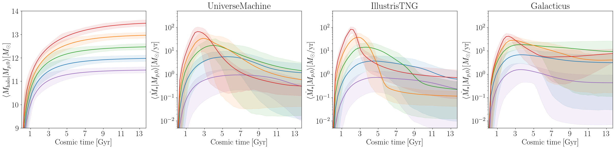
Compare SFHs for DiffstarPop params fitted to different simulations.

Here we plot the average SFHs using the best-fit diffstarpop values obtained from different simulations.

fig, ax = plt.subplots(1,4, figsize=(30,6), sharex=True)
mpeak_vals = np.arange(11.5, 14, 0.5)

for i, mpeak in enumerate(mpeak_vals):
    sel = (subcat.logmp0 > mpeak - 0.2) & (subcat.logmp0 < mpeak + 0.2)
    mean_log_mah_fit = np.mean(log_mah_fit[sel], axis=0)
    range_log_mah_fit = np.percentile(log_mah_fit[sel], [15.865, 84.135], axis=0)

    ax[0].plot(tarr, mean_log_mah_fit, color=colors[i])
    ax[0].fill_between(tarr, range_log_mah_fit[0], range_log_mah_fit[1],
                       color=colors[i], alpha=0.1)

for k, params in enumerate([DIFFSTARPOP_UM, DIFFSTARPOP_TNG, DIFFSTARPOP_GALCUS]):
    # compute SFHs for the default galaxy population
    args = (
        params,
        subcat.mah_params,
        subcat.logmp0,
        subcat.upids,
        lgmu_infall,
        logmhost_infall,
        gyr_since_infall,
        ran_key,
        tarr,
    )

    (
        diffstar_params_ms,
        diffstar_params_q,
        default_sfh_ms,
        default_sfh_q,
        frac_q,
        mc_is_q,
    ) = mc_diffstar_sfh_galpop(*args, lgt0=DEFAULT_LGT0, fb=DEFAULT_FB)

    default_sfh = np.zeros_like(default_sfh_ms)
    default_sfh[mc_is_q] = default_sfh_q[mc_is_q]
    default_sfh[~mc_is_q] = default_sfh_ms[~mc_is_q]

    for i, mpeak in enumerate(mpeak_vals):
        sel = (subcat.logmp0 > mpeak - 0.2)
        sel = sel & (subcat.logmp0 < mpeak + 0.2)
        mean_default_sfh = np.mean(default_sfh[sel], axis=0)
        range_mean_default_sfh = np.percentile(
            default_sfh[sel], [15.865, 84.135], axis=0)

        ax[k+1].plot(tarr, mean_default_sfh, color=colors[i])
        ax[k+1].fill_between(
            tarr, range_mean_default_sfh[0], range_mean_default_sfh[1],
            color=colors[i], alpha=0.1)


ax[0].set_ylim(9, 14)
ax[0].set_xticks(np.arange(1.0, 14.0, 2.0))
ax[0].set_xlabel("Cosmic time [Gyr]")
ax[1].set_xlabel("Cosmic time [Gyr]")
ax[2].set_xlabel("Cosmic time [Gyr]")
ax[3].set_xlabel("Cosmic time [Gyr]")
ax[0].set_xlim(0.0, 13.7)

ax[1].set_yscale('log')
ax[2].set_yscale('log')
ax[3].set_yscale('log')
ax[1].set_ylim(5e-3, 5e2)
ax[2].set_ylim(5e-3, 5e2)
ax[3].set_ylim(5e-3, 5e2)
ax[0].set_ylabel(r"$\langle M_{\rm halo} | M_{p,0} \rangle [M_{\odot}]$")
ax[1].set_ylabel(r"$\langle \dot{M}_\star | M_{p,0} \rangle [M_{\odot}/{\rm yr}]$")
ax[2].set_ylabel(r"$\langle \dot{M}_\star | M_{p,0} \rangle [M_{\odot}/{\rm yr}]$")
ax[3].set_ylabel(r"$\langle \dot{M}_\star | M_{p,0} \rangle [M_{\odot}/{\rm yr}]$")

ax[1].set_title("UniverseMachine")
ax[2].set_title("IllustrisTNG")
ax[3].set_title("Galacticus")

fig.subplots_adjust(wspace=0.25)


plt.show()